AP-COMP 221: Critical Thinking in Data Science

Abstract

We investigate how credit-scoring systems might disproportionately impact vulnerable groups in receiving loans and credit lines by assessing their use of different sensitive demographic attributes (age, gender, marital status, education). Using a dataset of credit default behavior of Taiwanese credit card holders, we implemented three machine learning methods commonly used in literature for credit default studies (logistic regression, random forest, kNN), trained once on the set of features, and then on the set of features with the sensitive attributes removed. We find that there are negligible difference in accuracy for the models with and without sensitive attributes, raising questions of why these sensitive attributes were collected in the first place. We further find that our classifier exhibits disparate impact bias, erroneously flagging people with a high school education as likely to default more often than people with higher degrees.

Introduction

Much of the recent success of machine learning in a number of domains has been attributed to the emergence of large datasets, giving rise to adages such as “the more data, the better.” Accordingly, providers of prediction services, notably credit-scoring companies, have broadened the range of information they use to construct their models. At the same time, algorithmic decision-making systems in high-stakes scenarios have attracted increased scrutiny, as civil society and academia have raised concerns about algorithmic bias.

In this paper, we investigate how credit-scoring systems that make use of a number of sensitive demographic attributes might disproportionately impact vulnerable groups in receiving loans and credit lines, by analyzing dataset of default behavior of Taiwanese credit-card holders.

In the United States, the Equal Credit Opportunity Act (ECOA) enacted by Congress in 1974 prohibits credit discrimination based certain protected categories, such as race, age, or marital status [1,2]. While this information may be collected by creditors, it cannot be used in order to make decisions about whether to offer credit, or to determine the terms of the credit. ECOA applies to decisions made by algorithms just as much as to those made by people.

Yet, as economic status is known to be heavily correlated with protected attributes, such as race, ECOA expectedly does not remove all differences in treatment between subpopulations when it comes to loan refusals, credit card limits, etc. Women in the United States, for example, tend to have lower credit limits than men, due to the gender gap in annual income. Consequently, they tend to spend a higher percentage of their credit limit, which in turn negatively impacts their credit score. [3] This phenomenon could therefore easily lead to runaway feedback loops that entrench existing inequalities. It is an instance of disparate impact, where a "formally neutral" system adversely affects certain groups of people without its designers having explicitly intended such outcomes.

In order to understand the role of protected attributes in credit scoring and to assess the potential of disparate impact of credit-scoring algorithms, we examine a credit-default dataset published by Yeh et al. in 2009 [4], which features both sensitive demographic attributes (gender, marital status, age, education) and payment behavior information, as well as the target variable of whether a person has defaulted on their credit or not. We assess the predictive performance of three commonly used classification models: logistic regression, random forest, and k-nearest neighbors which we train on (A) the set of all features and (B) on the set of features excluding sensitive attributes. In a second step, we determine whether the prediction quality of the best-performing classifier differs for different subpopulations who share a sensitive attribute. Finally, we discuss our results in the context of more general considerations on computational bias and data collection practices.

Background

Credit scores have become an increasingly important part of people’s economic life, as they are used as a basis for many activities and services, from buying a house and leasing a car, to insurance rates or employment [5, 6]. If a person is predicted to be at high risk for defaulting and therefore does not get access to the credit they need, they might not qualify for a home loan, have difficulty in paying unplanned expenses (for example, an urgent medical issue), and in general have their financial stability threatened. As automatic prediction systems increasingly mediate such credit-scoring decisions, it is crucial to understand and mitigate the risk of reinscribing and calcifying historical discriminatory practices.

Previous research is divided on whether credit scoring has a disparate impact on marginalized groups or not. A 2012 analysis of the National Fair Housing Alliance claims that not only do credit scores not accurately predict default rates but also that they disproportionately impact communities of color [7]. As mentioned above, other studies show a disparate impact of credit scoring on women compared to men [3]. However, another paper claims no evidence of disparate impact by race or gender, but limited disparate impact by age, where older individuals are at a disadvantage [8].

The dataset which we analyze in this paper was selected due to its popularity: Hosted on the UCI machine repository, almost 350,000 web hits were recorded, 182 notebooks have been shared by data science practitioners on Kaggle, and 266 scientific papers cite the initial paper, according to Google Scholar. When reviewing this literature, we were shocked to find that little to none of the published research critically engages with the potential for discriminatory predictions. Gender and marital status, in fact, are claimed to be strong predictors in several of the proposed models [4] without any critical thought concerning their use. We further found no papers that explicitly address disparate impact or even the question of whether the inclusion of sensitive attributes was beneficial for predictive performance.

We thus plan to contribute to the literature not only by assessing disparate impact on common algorithms in default predictions but also by analyzing whether accuracy is truly lost when algorithms do not use protected attributes. The latter question is important since governance debates about the use of personal information often center around a supposed trade-off between accuracy and utility of the system and privacy of the data subjects.

Methods: 1. Describing the Data

The dataset comprises 30,000 observations, each describing a unique credit-card account holder in Taiwan in September, 2005. The explanatory variables include sensitive attributes (gender, age, marital status, education), as well as the account holder’s payment behavior for the preceding six months (repayment status, amount of bill statement, amount of previous payment). A binary variable denotes whether the credit card owner defaulted (1) on their loan or not (0). Within the sample, the rate of default payment is 22.12%.

Credit limit	amount of credit offered to the credit card owner.
Gender	gender of the credit card holder; categories: male (1) or female (2).
Education	educational attainment of the credit card holder; categories: graduate school (1), university (2), high school (3), others (0, 4, 5, 6).
Marital status	marital status of the credit card holder; categories: married (1), single (2), divorced (3), others (0).
Age	age of the credit card holder.
History of payment	payment records for the previous 6 months, from April to September; categories: no consumption (-2), paid in full (-1), use of revolving credit (0), payment delay for one month (1), payment delay for 2 months (2), etc.
Amount of bill statement	amount of bill statements for the previous six months.
Amount of previous payment	amount of payment for bills in the previous six months.
Default	1 if the person defaulted on their payment, 0 otherwise.

Methods: 2. Exploratory Data Analysis

A common observation in the field of algorithmic fairness is that the data used to train algorithmic decision-making systems already encodes outcomes of various historical discriminatory practices. Therefore a simple question worth asking is who is missing in this dataset. To this end, we compared the distributions of several demographic attributes in the dataset to that of the Taiwanese population overall.

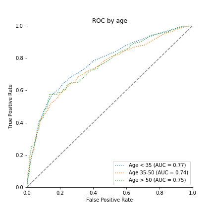
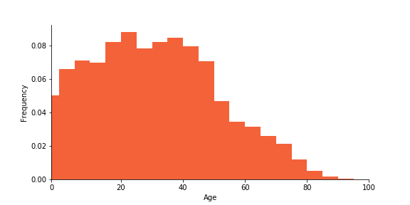
Age distribution of Taiwanese population

Age distribution of the credit data

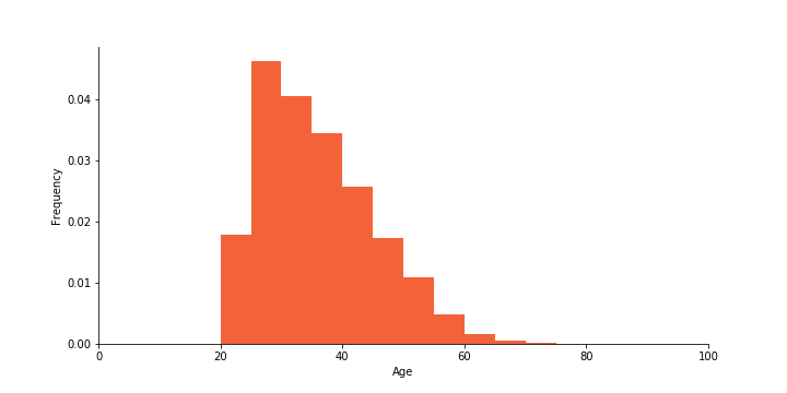
The people who are found in the credit card data are adults who tend to be younger than the general Taiwanese population. Especially elderly citizens are not represented. When faced with a new, unseen credit-card holder who is 70 or older, an automated decision-making system, such as one powered by logistic regression, may therefore likely extrapolate rather than interpolate from seen data.

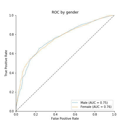
Gender presentation of Taiwanese population

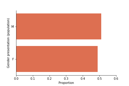
Gender presentation of the credit data

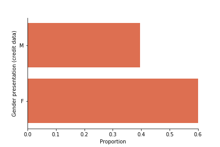
Women are overrepresented in the dataset. Further, the dataset’s M/F ontology reinscribes problematic binarized notions of gender, non-binary people are erased. [9]

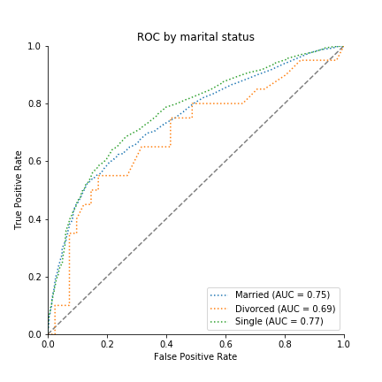
Marital Status of Taiwanese population

Marital Status of the credit data

While the majority of the Taiwanese population is married, the majority of the people represented in the credit dataset are single. The data further includes a disproportionately small number of divorced individuals. Widowed citizens are not represented explicitly in the credit data ontology.

Methods: 3. Transformations

Inspecting the data, we also notice that some values of certain variables were undocumented (education: 0, 4, 5, 6; marital status: 0) prompting us to remove all observations including such values, resulting in a final count of 29480 observations (98.26% of original data). The removal of these observations does not meaningfully change the marginal distributions of the dataset’s features. Furthermore, we transform the “history of payment” variable, which in its original form encoded both ordinal and categorical information, for the purposes of model interpretability. Investigating options with both a categorical variable for the “no_delay” value in payment subgroups and a continuous variable to measure the delay payments, we concluded that in terms of both model interpretability and performance, it was best to lump the no-delay categories into only one (0). Thus, our new history of payment attribute is described by:

History of payment: payment records for the previous 6 months, from April to September; categories: no delay (0), payment delay for one month (1), payment delay for 2 months (2), etc.

Finally, we convert the categorical variables gender, education, and marital status into one-hot encodings.

Methods: 4. Modeling

In order to examine how computational bias may be present in the models proposed in literature, we train and evaluate classifiers on two sets of features: (A) a feature set comprising all features, and (B) a feature set that excludes sensitive attributes. By comparing the predictive performance of models trained on (A) with that of models trained on (B), we can determine whether any accuracy is lost via the exclusion of sensitive variables. We split the dataset uniformly at random into training and validation sets with a 80/20 ratio, retaining the label proportions.

We train three models, tuning hyperparameters separately for each of the feature sets:

Logistic regression as a baseline and an interpretable parametric model
K-nearest neighbors as a nonparametric model
Random forest as a parametric model that we expected to reach high predictive power in practice with little parameter tuning

In a second step, to examine disparate impact, we choose the best-performing classifier on feature set (B) and inspect its ROC curves for the following subpopulations:

Gender (m, f)
Age (younger than 35, 35-50, older than 50)
Marital status (single, married, divorced)
Educational attainment (highschool, university, graduate school)

Results: 1. Model Accuracy and Interpretation

The performance of the fitted models in terms of AUC, precision, recall and F1 scores are summarized in the table below. F1 score, rather than accuracy, was chosen as an additional figure of merit due to the aforementioned unbalanced label distribution.

Model Performance

Model Type	AUC (A)	AUC (B)	F1-Score (A)	F1-Score (B)
Logistic Regression	0.7624	0.7478	0.78	0.78
kNN	0.6151	0.6190	0.72	0.72
Random Forest	0.7635	0.7570	0.79	0.79

For both feature sets, the best performing model in terms of the F1 score is random forest, matching our expectations and kNN is the worst performing model. Interestingly, there is no significant difference in overall performance between random forest and logistic regression; in fact, logistic regression in both cases has a higher F1 score for the “default” category than for the “no-default” category.

Logistic Regression Coefficients

Feature	Coefficient (A)	Coefficient (B) w/o sensitive attributes
age	0.0000	-
gender_male	0.1058	-
education_grad	0.0000	-
education_univ	0.0000	-
marriage_married	0.1362	-
marriage_divorced	0.0000	-
delay_0	0.8901	0.5892
delay_2	0.0833	0.0359
delay_3	0.1542	0.0280
delay_4	0.1025	0.0000
delay_5	0.1122	0.0000
delay_6	0.1214	0.0000
all others (limit_bal, bill_amount_0, ..., pay_amount_6)	0.0000	0.0000

Interpreting the coefficients of the logistic regression on feature set A, the most important features are, in order of importance, the payment delay for the most recent month, third month, being married, being male, and lastly the payment delays for the other months (all positive). All other attributes have coefficients of 0, due to L1 regularization which we found to outperform L2 regularization. Intuitively, payment delays in recent months are more predictive of a person defaulting than in months further in the past. The model does make use of sensitive attributes, where being male (gender) and being married (marital status) correlate with an individual being more likely to default on their credit. Deploying such a model would be illegal according to ECOA.

In a similar analysis of the feature importance statistics in random forest we notice that the payment delay for the most recent month has the highest feature importance, but is followed by the bill amount for the most recent month, and only then by the age of the credit owner, the credit limit, etc. Different from logistic regression, being married or being male have some of the lowest feature importance scores. This may be explained by the ability of random forest to model non-linearities in the data.

Excluding sensitive attributes in feature set B, the only variables with non-zero coefficients in logistic regression are the payment delays for the previous 3 months (again, in decreasing order of coefficient magnitude as we go backwards in time). For random forest without sensitive attributes, the variables with the highest coefficients are the bill amount for the most recent month, the payment delay for the most recent month, the credit limit etc. There are only minor differences in terms of these scores and their order compared to the random forest with sensitive attributes.

Receiver Operating Characteristic Curve

Based on the results summarized above, we note that there is a very small difference in terms of performance between each method on the feature sets with sensitive attributes (A) and without sensitive attributes (B). The performance of the logistic regression and of the random forest in terms of the AUC is not significantly worse, while for kNN, the AUC actually increases when we exclude the sensitive variables. Our results suggest that, in this particular case, removing sensitive attributes would result in negligible performance degradation.

Results 2: Disparate Impact

We select the random forest model trained on feature set B (the best model) in order to analyze its potential for disparate impact.

Gender, Age, Marital Status

The classifier does not perform significantly differently for subpopulations along the lines of gender, marital status, and age. (“divorced” for marital status had only few samples (<100), resulting in the jagged ROC curve). We do not notice any major discrepancies in false positive or true positive rates based on the sensitive categories.

Education

The classifier underperforms when making predictions for people with high school degrees as their highest educational attainment for thresholds with true positive rates > 0.6. Therefore, the high-school subpopulation would be erroneously flagged by an automatic decision-making system more often than other people with higher degrees.

Discussion

Overall, there were no major differences in terms of model performance (AUC) between the methods that used sensitive attributes and those that did not. This disproves the common narrative of there being a trade-off between accuracy and privacy/bias.

Both the risk of legal exposure for failing to protect this sensitive data and the long-term engineering benefits of keeping ML pipelines simple lead us to believe that it would be rational to minimize data collection. Age, education, gender and marital status are all quasi-identifiers, which in combination with other data might allow for the re-identification of the subjects in the dataset, and consequently the revealing of sensitive financial data associated with them. Including the variables in the dataset could also lead to human bias (even if it is implicit) for decision makers who would have access to the prediction, as well as to the rest of the profile of the subject. In our view, the only ethically justifiable reason for collecting these sensitive attributes would be for purposes of investigating algorithmic bias. However, our literature review has shown this not to be the case in practice.

Concerning model selection, we would advise the use of logistic regression due to its interpretable characteristics and quick optimization procedure that can be harnessed without sacrificing much predictive power.

In our disparate impact analysis, we find no evidence of bias against subpopulations that share a certain age, gender or marital status, which are protected categories in the US. In terms of level of education, we find a difference in performance for people with high school degrees. This might be problematic due to the fact that lower educational attainment is known to correlate with lower income, and thus we might be denying people who are at low risk of defaulting the credit they might be needing more than higher income populations. However, bias need not be the reason for the inferior performance. Maybe the economic trajectories of people whose highest educational degree is high school are more random / have higher variability than those of people with higher educational degrees, making them harder to predict. More research and inquiry into the dataset is needed to address such questions.

Additionally, it is worth asking to what extent a US dataset would differ from the Taiwan one: would the same variables be the most important ones, would using sensitive attributes such as race make a bigger difference in accuracy, etc. Further research could focus on possible comparisons between models trained on different datasets.

Further possible avenues of research could be the following:

1. Feedback Loop Simulation

As mentioned above, a widely discussed issue in credit score assessment is the presence of feedback loops. If you are an individual who is initially denied for a loan or credit card line, then you might face additional financial hardships, such as not being able to purchase a home or car, or pay for unexpected costs. This might, in turn, negatively impact your credit score, making it even less likely for you to get further loans. This kind of feedback loops can also be seen in predictive policing, as described in a 2018 paper by Ensign et al. [10]. Employing a similar methodology, we would like to create simulations to prove the existence of such feedback loops, as well as possible interventions.

2. Categorizing practicioner's errors

As previously mentioned, many Kaggle users and papers have done work with this dataset. While investigating issues with unexplained categories (that we managed to get explanations for directly from the author of the original paper), we noticed several types of errors that were being made in the analysis, either in terms of the technical aspects of the models employed, or in the interpretation of the results. We aim to look at a larger number of these papers/notebook and create a classification for the most common type of errors, and discuss their implications.

References

Find our Github repository here.
[1] Federal Trade Commission. (n.d.) Your Equal Credit Opportunity Rights. Retrieved from https://www.consumer.ftc.gov/articles/0347-your-equal-credit-opportunity-rights.
[2] Hurley, M., Adebayo, J. (2017). Credit Scoring in the Era of Big Data. Yale Journal of Law and Technology 18(1).
[3] Mayer, C. (November 10, 2017). How Does Gender Affect Credit Scores? Fiscal Tiger. Retrieved from https://www.fiscaltiger.com/gender-affect-credit-scores/.
[4] Yeh, I-C., Lien, C. (2009). The comparisons of data mining techniques for the predictive accuracy of probability of default of credit card clients. Expert Systems with Applications 36(2): 2473-2480.
[5] Ortiz, L.M. (July 25, 2016). Challenging the Almighty Credit Score. Shelterforce. Retrieved from https://shelterforce.org/2016/07/25/challenging-the-almighty-credit-score/.
[6] Pritchard, J. (March 11, 2018). What is Credit? The Balance. Retrieved from https://www.thebalance.com/what-is-credit-315391.
[7] Rice, L., Swesnik, D. (June, 2012). Discriminatory Effects of Credit Scoring on Communities of Color. National Fair Housing Alliance. Retrieved from https://nationalfairhousing.org/wp-content/uploads/2017/04/NFHA-credit-scoring-paper-for-Suffolk-NCLC-symposium-submitted-to-Suffolk-Law.pdf
[8] Avery, R.B., Brevoort, K.P., Canner, G.B. Does Credit Scoring Produce a Disparate Impact? Federal Reserve. Retrieved from https://www.federalreserve.gov/pubs/feds/2010/201058/201058pap.pdf.
[9] Keyes, Os. The Misgendering Machines: Trans/HCI Implications of Automatic Gender Recognition. Retrieved from https://ironholds.org/resources/papers/agr_paper.pdf.
[10] Ensign, D., Friedler, S.A., Neville, S., Scheidegger, C., Venkatasubramanian, S. (2018). Runaway Feedback Loops in Predictive Policing. Proceedings of Machine LEarning Research 81: 1-12.